RLEQU
Fits a multivariate linear regression model with linear equality restrictions H B = G imposed on the regression parameters given results from routine RGIVN after IDO = 1 and IDO = 2 and prior to IDO = 3.
Required Arguments
H — NH by NCOEF matrix with the i-th row specifying a linear combination of the regression parameters for the i-th row in the restriction H B = G. (Input)
B — NCOEF by NDEP matrix containing on return from the final invocation of this routine a least-squares solution for the regression coefficients in the restricted model. (Input/Output)
Invocation of RLEQU with INVOKE = 0 and 1 requires as input the B matrix from RGIVN after RGIVN’s invocation with IDO = 1 and IDO = 2 and prior to IDO = 3 with NROW = 0. After the wrap-up computations are computed by RLEQU, B contains a least-squares solution for the regression coefficients in the restricted model.
Invocation of RLEQU with INVOKE = 0 and 1 requires as input the B matrix from RGIVN after RGIVN’s invocation with IDO = 1 and IDO = 2 and prior to IDO = 3 with NROW = 0. After the wrap-up computations are computed by RLEQU, B contains a least-squares solution for the regression coefficients in the restricted model.
R — NCOEF by NCOEF upper triangular matrix containing, on return from the final invocation of this routine, the R matrix from the restricted regression fit. (Input/Output)
Invocation of RLEQU with INVOKE = 0 and 1 requires as input the R matrix from RGIVN after RGIVN’s invocation with IDO = 1 and IDO = 2 and prior to IDO = 3 with NROW = 0. After the wrap-up computations are computed by RLEQU, R contains the R matrix from the restricted regression fit. Elements to the right of a diagonal element of R (that is zero) are also zero. A zero row in R indicates a nonfull rank model. Each row of R corresponding to a restriction has a corresponding diagonal element that is negative. Each remaining row of R has a corresponding diagonal element that is positive.
Invocation of RLEQU with INVOKE = 0 and 1 requires as input the R matrix from RGIVN after RGIVN’s invocation with IDO = 1 and IDO = 2 and prior to IDO = 3 with NROW = 0. After the wrap-up computations are computed by RLEQU, R contains the R matrix from the restricted regression fit. Elements to the right of a diagonal element of R (that is zero) are also zero. A zero row in R indicates a nonfull rank model. Each row of R corresponding to a restriction has a corresponding diagonal element that is negative. Each remaining row of R has a corresponding diagonal element that is positive.
D — Vector of length NCOEF containing scale factors associated with the fast Givens transformations. (Input/Output)
Invocation of RLEQU with INVOKE = 0 and 1 requires as input the D from RGIVN after RGIVN’s invocation with IDO = 1 and IDO = 2 and prior to IDO = 3 with NROW = 0. After the wrap-up computations are computed by RLEQU, D contains all its elements set to 1.0.
Invocation of RLEQU with INVOKE = 0 and 1 requires as input the D from RGIVN after RGIVN’s invocation with IDO = 1 and IDO = 2 and prior to IDO = 3 with NROW = 0. After the wrap-up computations are computed by RLEQU, D contains all its elements set to 1.0.
DFE — Degrees of freedom for error for the restricted model on return from the final invocation of this routine. (Input/Output)
Prior to the final invocation of this routine, DFE contains the sum of the frequencies. Invocation of RLEQU with INVOKE = 0 and 1 requires as input the DFE from RGIVN after RGIVN’s invocation with IDO = 1 and IDO = 2 and prior to IDO = 3 with NROW = 0.
Prior to the final invocation of this routine, DFE contains the sum of the frequencies. Invocation of RLEQU with INVOKE = 0 and 1 requires as input the DFE from RGIVN after RGIVN’s invocation with IDO = 1 and IDO = 2 and prior to IDO = 3 with NROW = 0.
SCPE — NDEP by NDEP matrix containing error (residual) sums of squares and crossproducts for the restricted model. (Input/Output)
SCPE(M, N) is the current sum of crossproducts of residuals for the M-th and N-th dependent variables. Invocation of RLEQU with INVOKE = 0 and 1 requires as input the SCPE matrix from RGIVN after RGIVN’s invocation with IDO = 1 and IDO = 2 and prior to IDO = 3 with NROW = 0.
SCPE(M, N) is the current sum of crossproducts of residuals for the M-th and N-th dependent variables. Invocation of RLEQU with INVOKE = 0 and 1 requires as input the SCPE matrix from RGIVN after RGIVN’s invocation with IDO = 1 and IDO = 2 and prior to IDO = 3 with NROW = 0.
Optional Arguments
INVOKE — Invocation option. (Input)
Default: INVOKE = 0.
Default: INVOKE = 0.
INVOKE | Action |
0 | This is the only invocation of RLEQU. All the restrictions are input at once. |
1 | This is the first invocation, and additional calls to RLEQU will be made. Initialization and updating for the restrictions H B = G are performed. |
2 | This is an intermediate invocation of RLEQU, and updating for the restrictions H B = G is performed. |
3 | This is the final invocation of this routine. Updating for the restrictions H B = G is performed, and wrap-up computations are performed. |
NH — Number of rows in the restriction H B = G. (Input)
Default: NH = size (H,1).
Default: NH = size (H,1).
NCOEF — Number of coefficients in the regression equation for each dependent variable. (Input)
Default: NCOEF = size (H,2).
Default: NCOEF = size (H,2).
LDH — Leading dimension of H exactly as specified in the dimension statement of the calling program. (Input)
Default: LDH = size (H,1).
Default: LDH = size (H,1).
IG — Option for G matrix. (Input)
Default: IG = 0.
Default: IG = 0.
IG | Restrictions |
|---|---|
0 | H B = 0 |
1 | H B = G |
NDEP — Number of dependent (response) variables. (Input)
Default: NDEP = size (B,2).
Default: NDEP = size (B,2).
G — NH by NDEP matrix containing the right-hand side of the restriction
H B = G. (Input, if IG = 1)
If IG = 0, G is not referenced and can be a 1 by 1 array.
Default: G is a 1 by 1 array.
H B = G. (Input, if IG = 1)
If IG = 0, G is not referenced and can be a 1 by 1 array.
Default: G is a 1 by 1 array.
LDG — Leading dimension of G exactly as specified in the dimension statement in the calling program. (Input)
Default: LDG = size(G, 1).
Default: LDG = size(G, 1).
TOL — Tolerance used in determining linear dependence. (Input)
For RLEQU, TOL = 100.0 * AMACH(4) is a common choice. See the documentation for IMSL routines AMACH in Reference Material.
Default: TOL = 1.e-5 for single precision and 2.d-14 for double precision.
For RLEQU, TOL = 100.0 * AMACH(4) is a common choice. See the documentation for IMSL routines AMACH in Reference Material.
Default: TOL = 1.e-5 for single precision and 2.d-14 for double precision.
LDB — Leading dimension B exactly as specified in the dimension statement in the calling program. (Input)
Default: LDB = size (B,1).
Default: LDB = size (B,1).
LDR — Leading dimension of R exactly as specified in the dimension statement in the calling program. (Input)
Default: LDR = size (R,1).
Default: LDR = size (R,1).
IRANKR — Rank of matrix R. (Output, if INVOKE = 0 or 3)
LDSCPE — Leading dimension of SCPE exactly as specified in the dimension statement in the calling program. (Input)
Default: LDSCPE = size (SCPE,1).
Default: LDSCPE = size (SCPE,1).
IRANKH — Rank of matrix H. (Output)
FORTRAN 90 Interface
Generic: CALL RLEQU (H, B, R, D, DFE, SCPE[, …])
Specific: The specific interface names are S_RLEQU and D_RLEQU.
FORTRAN 77 Interface
Single: CALL RLEQU (INVOKE, NH, NCOEF, H, LDH, IG, NDEP, G, LDG, TOL, B, LDB, R, LDR, D, IRANKR, DFE, SCPE, LDSCPE, IRANKH)
Double: The double precision name is DRLEQU.
Description
Routine RLEQU requires the output from routine RGIVN after RGIVN has been invoked with IDO = 1 and IDO = 2 and prior to IDO = 3 with NROW = 0. Similarly, RLEQU can use results from IMSL routine RGLM.
The routine RLEQU is designed so that you can partition a large number of restrictions, as might arise in classification models, into several groups of restrictions (each requiring less space) and make multiple calls to RLEQU (with INVOKE = 1, 2, 2, …, 3). Alternatively, one invocation of RLEQU (with INVOKE = 0) can be made with all the restrictions contained in H and G.
After the wrap-up computations are performed by RLEQU, routines RSTAT and RCASE can be used to compute and print summary statistics and case statistics related to the fitted regression.
Routine RGIVN (or RGLM) together with routine RLEQU compute estimates of the regression coefficients in a multivariate general linear model Y = X B + Ε subject to H B = G. Here, Y is the n × q matrix of responses, X is the n × p matrix of regressors, B is the p × q matrix of regression coefficients, and Ε is the n × q matrix of errors whose q-dimensional rows are identically and independently distributed multivariate normal with mean vector 0 and variance-covariance matrix Σ. The restriction is specified by the h × p matrix H and the h × q matrix G.
Previously, algorithms for solving the restricted least-squares problem were based on solving the following equations (Rao, 1973, page 232):
Routine RLEQU is based on an orthogonal reduction of X to upper triangular form. Fast Givens transformations with modifications described by Stirling (1981) for incorporating restrictions are used. This method has two main advantages: (1) the loss of accuracy resulting from forming XT X and XT Y is avoided, and (2) restrictions can be conveniently added so as to take advantage of the previous computations performed.
The method conceptually treats restrictions as observations with zero error variance. Fast Givens transformations as described by Golub and Van Loan (1983, pages 156‑162) are used. The modification to the matrix R from the unrestricted fit to form a modified
for the restricted fit is as follows:
1. If the leading nonzero element of the first restriction is small (as determined by TOL times a computed scale factor), the element is set to zero.
2. Let i be the index of the leading nonzero element in the modified first restriction. Replace row i of R by the restriction. Flag the i-th row as a restriction. Use the restriction to reduce the first nonzero element of the row that was removed from R to zero. Incorporate the row that has been reduced by the restriction into the remaining rows of R as if it were new data.
3. Add additional restrictions into R by using Gaussian elimination, with the rows in R corresponding to restrictions, to reduce the restriction to a form so that it can replace a row of R corresponding to data and preserve the upper triangular structure of R. While performing the Gaussian elimination, set small nonzero elements (as determined by TOL times a computed scale factor) of the reduced restriction to zero, so that errors from inexact computer arithmetic are not incorporated as a new restriction. Flag the row as a restriction. Use the restriction to reduce the first nonzero element of the row that was removed from R to zero. Incorporate the row that has been reduced by the restriction into the remaining rows of R as if it were new data.
4. After all the data and restrictions are incorporated, the i-th row of R (where i ranges over each row of R corresponding to a linearly independent constraint) is used to zero out elements of R in the i-th column of the previous rows of R that correspond to data. Although this step is not required to get a least-squares solution, Sallas (1988) recommends this step so that the rows and columns of
corresponding to data form the R matrix for the reduced model that arises from expressing some regression parameters, βi, in terms of other regression parameters, βj(j > i).
Linear dependence of the regressors in the reduced model is then checked as part of the wrap-up computations, using the rows and columns of R corresponding to the reduced model. The check is complicated somewhat by the fact that a regressor could become zero in the reduced model, but because of the finite precision of computer arithmetic, the regressor is not exactly zero. Let di equal the i-th diagonal element of XT X, and let
equal the corresponding diagonal from the crossproducts matrix for the reduced model. Linear dependence of regressors in the reduced model is declared if
is less than or equal to TOL or if
is less than or equal to TOL. (The last check is designed to detect a zero regressor in the reduced model.) Here,
is the square of the “multiple correlation” coefficient of the i-th regressor in the reduced model with the first i ‑ 1 regressors in the reduced model. The “multiple correlation” coefficient is computed using the regressors in the reduced model and adjusted for the mean only if the incorporated restrictions have that effect.
When a linear dependence is declared, R is changed so as to reflect the deletion of the i-th regressor from the model. On completion of the wrap-up computations, the rows of R can be partitioned into three classes according to the sign of the corresponding diagonal element:
1. A positive diagonal element means the row/column corresponds to data for regressors in the reduced model.
2. A negative diagonal element means the row corresponds to a linearly independent restriction imposed on the regression parameters by H B = G.
3. A zero diagonal element means a linear dependence in the reduced model was declared. The regression coefficients in the corresponding row of
are set to zero. This represents an arbitrary restriction that is imposed to obtain a solution for the regression coefficients. The elements of the corresponding row of R are also set to zero.
Redundant restrictions on the regression parameters are frequently specified in general linear models. Routine RLEQU permits redundant restrictions and returns the rank of H. An informational error is issued if inconsistent restrictions are detected.
Comments
1. Workspace may be explicitly provided, if desired, by use of R2EQU/DR2EQ. The reference is:
CALL R2EQU (INVOKE, NH, NCOEF, H, LDH, IG, NDEP, G, LDG, TOL, B,LDB, R, LDR, D, IRANKR, DFE, SCPE, LDSCPE, IRANKH, WK)
The additional argument is:
WK — Work vector of length NCOEF + NDEP.
2. Informational error
Type | Code | Description |
|---|---|---|
3 | 1 | The restrictions are inconsistent. |
3. The results of routine RGLM can be used as input to RLEQU in place of the results of routine RGIVN.
Examples
Example 1
A grafted polynomial (spline function) is fit to data discussed by Fuller (1976, pages 396‑398). The data set contains the response variable y measuring the annual wheat yield (in bushels per acre) for the years 1908 through 1971. In order to fit the trend, Fuller fits a function that is constant for the first 25 years, increases at a quadratic rate until 1961, and is linear for the last 10 years. This trend is represented by the function f(t) where
where t = 1 for 1908.
In order to fit a smooth function to the data, we require both continuity and differentiability. This imposes four restrictions on the coefficients given as follows:
1. β1 ‑ β2 ‑ 25 β3 ‑ 252 β4 = 0
2. β2 + 54 β3 + 542 β4 ‑ β5 ‑ 54 β6 = 0
3. β3 + 50 β4 = 0
4. β3 + 108 β4 ‑ β6 = 0
The example program first calls routine RGIVN with IDO = 1, which specifies that initialization and updating for the data are performed and wrap-up computations are not performed. This intermediate output from RGIVN along with the restrictions is the input to RLEQU .
USE IMSL_LIBRARIES
IMPLICIT NONE
INTEGER IDEP, LDB, LDG, LDH, LDR, LDSCPE, LDX, NCOEF, NH, &
NOBS, NVAR, J
PARAMETER (IDEP=1, LDG=1, NCOEF=6, NH=4, NOBS=64, NVAR=7, &
LDB=NCOEF, LDH=NH, LDR=NCOEF, LDSCPE=IDEP, LDX=NOBS)
!
INTEGER I, IDO, IG, INDDEP(IDEP), INDIND(NCOEF), INTCEP, &
IRANK, IRANKH, IRANKR, ICEN, NOUT, NRMISS
REAL B(LDB,IDEP), D(NCOEF), DFE, G(LDG,IDEP), &
H(LDH,NCOEF), R(LDR,NCOEF), SCPE(LDSCPE,IDEP), &
X(LDX,NVAR), XMAX(NCOEF), XMIN(NCOEF)
CHARACTER*4 RLABEL(1), CLABEL(1)
!
DATA INDIND/1, 2, 3, 4, 5, 6/, INDDEP/7/
DATA X/384*0.0, 14.3, 15.5, 13.7, 12.4, 15.1, 14.4, 16.1, 16.7, &
11.9, 13.2, 14.8, 12.9, 13.5, 12.7, 13.8, 13.3, 16.0, 12.8, &
14.7, 14.7, 15.4, 13.0, 14.2, 16.3, 13.1, 11.2, 12.1, 12.2, &
12.8, 13.6, 13.3, 14.1, 15.3, 16.8, 19.5, 16.4, 17.7, 17.0, &
17.2, 18.2, 17.9, 14.5, 16.5, 16.0, 18.4, 17.3, 18.1, 19.8, &
20.2, 21.8, 27.5, 21.6, 26.1, 23.9, 25.0, 25.2, 25.8, 26.5, &
26.3, 25.9, 28.4, 30.6, 31.0, 33.9/
DATA (H(1,J),J=1,NCOEF)/1, -1, -25, -625, 0, 0/
DATA (H(2,J),J=1,NCOEF)/0, 1, 54, 2916, -1, -54/
DATA (H(3,J),J=1,NCOEF)/0, 0, 1, 50, 0, 0/
DATA (H(4,J),J=1,NCOEF)/0, 0, 1, 108, 0, -1/
!
DATA RLABEL/'NONE'/,CLABEL/'NONE'/
!
DO 10 I=1, NOBS
IF (I .LE. 25) THEN
! Constant function.
X(I,1) = 1.0
ELSE IF (I.GT.25 .AND. I.LE.54) THEN
! Quadratic function.
X(I,2) = 1.0
X(I,3) = I
X(I,4) = I**2
ELSE IF (I .GT. 54) THEN
! Linear function.
X(I,5) = 1.0
X(I,6) = I
END IF
10 CONTINUE
IDO = 1
INTCEP = 0
ICEN = 0
CALL RGIVN (X, NCOEF, INDIND, IDEP, INDDEP, B, IDO=IDO, &
INTCEP=INTCEP, ICEN=ICEN, R=R, D=D, DFE=DFE, SCPE=SCPE)
CALL RLEQU (H, B, r, d, DFE, SCPE, irankr=irankr, Irankh=irankh)
CALL UMACH (2, NOUT)
WRITE (NOUT,*) 'IRANKR = ', IRANKR, ' IRANKH = ', IRANKH
WRITE (NOUT,*) 'DFE = ', DFE, ' SCPE(1,1) = ', SCPE(1,1)
CALL WRRRL ('%/B', B, RLABEL, CLABEL, 1, NCOEF, 1, FMT='(2W10.4)')
CALL WRRRL ('%/R', R, RLABEL, CLABEL, ITRING=1, FMT='(2W10.4)')
END
Output
IRANKR = 6 IRANKH = 4
DFE = 62.0000 SCPE(1,1) = 172.559
B
13.99 21.58 -0.6068 0.01214 -13.81 0.7039
R
-1 1 25 625 0. 0.0
-1 -54 -2916 1. 54.0
-1 -50 0. 0.0
-58 0. 1.0
8. 359.4
59.4
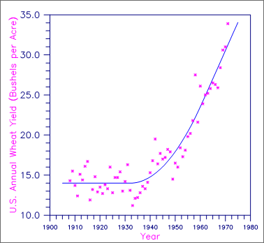
Figure 5, Annual U.S. Wheat Yield and a Grafted Polynomial Fit
Example 2
A fit to unbalanced data for a two-way classification model is computed. The model is
yijk = μ + α i+ βj+ γij + ɛ ijk i = 1, 2; j = 1, 2; k = 1, 2, …, nij
where the αi’s and βj’s are the row and column effects, respectively, and γij’s are the interaction effects. The responses yijk are given in the cells of the following 2 × 2 table:
17, 14, 11 | 13, 12 |
12, 14, 15, 14, 12 | 13, 14 |
The following restrictions can be imposed on the regression parameters in order to compute a cell-means fit to the responses:
1. 5 α1 + 7 α2 = 0
2. 8 β1 + 4 β2 = 0
3. 3 α1 + 5 α2 + 3 γ11+ 5 γ21 = 0
4. 2 α1 + 2 α2 + 2 γ12+ 2 γ22 = 0
5. 3 β1 + 2 β2 + 3 γ11+ 2 γ21 = 0
6. 5 β1 + 2 β2 + 5 γ12+ 2 γ22 = 0
The example program first calls IMSL routine RGLM with IDO = 1, which specifies that initialization and updating for the data are performed and wrap-up computations are not performed. This intermediate output from RGLM along with the restrictions is the input to RLEQU.
A cell-means fit to the data could also be obtained without using RLEQU and using IDO = 0 in the call to RGLM in this example. Although the fitted yijk would be the same, the coefficient estimates and their interpretations would be different.
USE IMSL_LIBRARIES
IMPLICIT NONE
INTEGER IDEP, INTCEP, LDB, LDG, LDH, LDR, LDSCPE, LDX, MAXCL, &
NCLVAR, NCOEF, NEF, NH, NOBS, NVAR, J
PARAMETER (IDEP=1, INTCEP=1, LDG=1, LDH=6, MAXCL=4, NCLVAR=2, &
NCOEF=9, NEF=3, NH=6, NOBS=12, NVAR=3, LDB=NCOEF, &
LDR=NCOEF, LDSCPE=IDEP, LDX=NOBS)
!
INTEGER IDO, INDCL(NCLVAR), INDDEP(1), INDEF(4),&
IRANK, IRANKH, IRANKR, IRBEF(NEF+1), ICEN, &
NCLVAL(NCLVAR), NOUT, NRMISS, NVEF(NEF)
REAL B(LDB,IDEP), CLVAL(MAXCL), D(NCOEF), DFE, &
G(LDG,IDEP), H(LDH,NCOEF), R(LDR,NCOEF), &
SCPE(LDSCPE,IDEP), X(LDX,NVAR), XMAX(NCOEF), &
XMIN(NCOEF)
CHARACTER CLABEL(10)*7, RLABEL(1)*4
!
DATA INDCL/1, 2/, NVEF/1, 1, 2/, INDEF/1, 2, 1, 2/, INDDEP/3/
DATA CLABEL/' ', 'MU', 'ALPHA1', 'ALPHA2', 'BETA1', 'BETA2', &
'GAMMA11', 'GAMMA12', 'GAMMA21', 'GAMMA22'/
DATA (X(1,J),J=1,NVAR) /1, 1, 17/
DATA (X(2,J),J=1,NVAR) /1, 1, 14/
DATA (X(3,J),J=1,NVAR) /1, 1, 11/
DATA (X(4,J),J=1,NVAR) /1, 2, 13/
DATA (X(5,J),J=1,NVAR) /1, 2, 12/
DATA (X(6,J),J=1,NVAR) /2, 1, 12/
DATA (X(7,J),J=1,NVAR) /2, 1, 14/
DATA (X(8,J),J=1,NVAR) /2, 1, 15/
DATA (X(9,J),J=1,NVAR) /2, 1, 14/
DATA (X(10,J),J=1,NVAR) /2, 1, 12/
DATA (X(11,J),J=1,NVAR) /2, 2, 13/
DATA (X(12,J),J=1,NVAR) /2, 2, 14/
DATA (H(1,J),J=1,NCOEF) /0, 5, 7, 0, 0, 0, 0, 0, 0/
DATA (H(2,J),J=1,NCOEF) /0, 0, 0, 8, 4, 0, 0, 0, 0/
DATA (H(3,J),J=1,NCOEF) /0, 3, 5, 0, 0, 3, 0, 5, 0/
DATA (H(4,J),J=1,NCOEF) /0, 2, 2, 0, 0, 0, 2, 0, 2/
DATA (H(5,J),J=1,NCOEF) /0, 0, 0, 3, 2, 3, 2, 0, 0/
DATA (H(6,J),J=1,NCOEF) /0, 0, 0, 5, 2, 0, 0, 5, 2/
!
IDO = 1
ICEN = 0
CALL RGLM (IDO=IDO, INDCL, NVEF, INDEF, IDEP, INDDEP, MAXCL, B, &
ICEN=ICEN, R=R, D=D, DFE=DFE, SCPE=SCPE)
CALL RLEQU (H, B, r, d, DFE, SCPE, irankr=irankr, &
irankh=irankh)
CALL UMACH (2, NOUT)
WRITE (NOUT,*) 'IRANKR = ', IRANKR, ' IRANKH = ', IRANKH
WRITE (NOUT,*) 'DFE = ', DFE, ' SCPE(1,1) = ', SCPE(1,1)
RLABEL(1) = 'NONE'
CALL WRRRL ('B', B, RLABEL, CLABEL, 1, NCOEF, 1, FMT='(F7.2)')
CALL WRRRN ('R', R, ITRING=1)
END
Output
IRANKR = 9 IRANKH = 5
DFE = 8.00000 SCPE(1,1) = 26.2000
B
MU ALPHA1 ALPHA2 BETA1 BETA2 GAMMA11 GAMMA12 GAMMA21
13.42 -0.02 0.01 0.21 -0.42 0.39 -0.48 -0.24
GAMMA22
0.49
R
1 2 3 4 5 6 7 8 9
1 3.46 0.00 0.00 0.00 0.00 0.00 0.00 0.00 0.00
2 -5.00 -7.00 0.00 0.00 0.00 0.00 0.00 0.00
3 -0.80 0.00 0.00 -3.00 0.00 -5.00 0.00
4 -8.00 -4.00 0.00 0.00 0.00 0.00
5 -0.50 -3.00 -2.00 0.00 0.00
6 -3.00 -2.00 -5.00 -2.00
7 10.41 3.20 11.37
8 24.56 9.65
9 2.45


