mlffNetworkForecast
Calculates forecasts for trained multilayered feedforward neural network.
Synopsis
mlffNetworkForecast (network, nominal, continuous)
Required Arguments
- Imsls_d_NN_Network
network(Input) - A Imsls_d_NN_Network containing the trained feedforward network. See mlffNetwork.
- int
nominal[](Input) - Array of size
nNominalcontaining the nominal input variables. - float
continuous[](Input) - Array of size
nContinuouscontaining the continuous input variables.
Return Value
An array of size nOutputs containing the forecasts, where nOutputs
is the number of output perceptrons in the network. nOutputs =
network.n_outputs.
Description
Function mlffNetworkForecast calculates a forecast for a previously
trained multilayered feedforward neural network using the same network
structure and scaling applied during the training. The structure
Imsls_d_NN_Network describes the network structure used to originally
train the network. The weights, which are the key output from training, are
used as input to this routine. The weights are stored in the
Imsls_d_NN_Network structure.
In addition, two one-dimensional arrays are used to describe the values of the nominal and continuous attributes that are to be used as network inputs for calculating the forecast.
Training Data
Neural network training data consists of the following three types of data:
- nominal input attribute data
- continuous input attribute data
- continuous output data
The first data type contains the encoding of any nominal input attributes. If binary encoding is used, this encoding consists of creating columns of zeros and ones for each class value associated with every nominal attribute. If only one attribute is used for input, then the number of columns is equal to the number of classes for that attribute. If more columns appear in the data, then each nominal attribute is associated with several columns, one for each of its classes.
Each column consists of zeros, if that classification is not associated with this case, otherwise, one if that classification is associated. Consider an example with one nominal variable and two classes: male and female (male, male, female, male, female). With binary encoding, the following matrix is sent to the training engine to represent this data:
Continuous input and output data are passed to the training engine using the
arrays: continuous and output. The number of rows in each of these
matrices is nPatterns. The number of columns in continuous and
output, corresponds to the number of input and output variables,
respectively.
Network Configuration
The configuration of the network consists of a description of the number of perceptrons for each layer, the number of hidden layers, the number of inputs and outputs, and a description of the linkages among the perceptrons. This description is passed into this forecast routine through the structure Imsls_d_NN_Network. See mlffNetwork.
Forecast Calculation
The forecast is calculated from the input attributes, network structure and weights provided in the structure Imsls_d_NN_Network.
Example
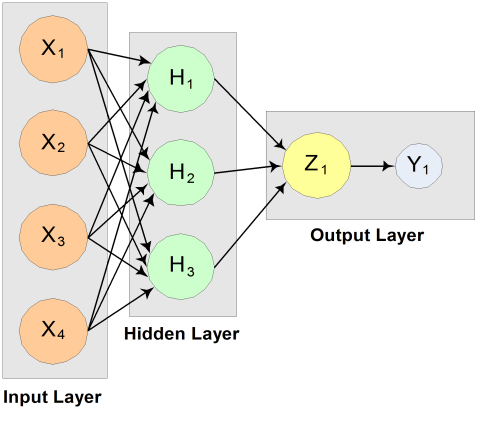
This example trains a two-layer network using 90 training patterns from one nominal and one continuous input attribute. The nominal attribute has three classifications which are encoded using binary encoding. This results in three binary network input columns. The continuous input attribute is scaled to fall in the interval [0,1].
The network training targets were generated using the relationship:
where \(X_1\), \(X_2\), \(X_3\) are the three binary columns, corresponding to the categories 1-3 of the nominal attribute, and \(X_4\) is the scaled continuous attribute.
The structure of the network consists of four input nodes ands two layers, with three perceptrons in the hidden layer and one in the output layer. The following figure illustrates this structure:

Figure 13.14 — A 2-layer, Feedforward Network with 4 Inputs and 1 Output
There are a total of 100 outputs. The first 90 outputs use
mlffNetworkTrainer to train the network and the
last 10 outputs use mlffNetworkForecast to forecast and compare the
actual outputs.
from __future__ import print_function
from numpy import *
from readMlffNetworkData import readMlffNetworkData
from pyimsl.stat.mlffNetwork import mlffNetwork
from pyimsl.stat.mlffNetworkFree import mlffNetworkFree
from pyimsl.stat.mlffNetworkInit import mlffNetworkInit
from pyimsl.stat.mlffNetworkTrainer import mlffNetworkTrainer
from pyimsl.stat.mlffNetworkForecast import mlffNetworkForecast
from pyimsl.stat.randomSeedSet import randomSeedSet
from pyimsl.stat.scaleFilter import scaleFilter

nominalObs = [0, 0, 0]
continuousObs = 0

nominal, continuous, output = readMlffNetworkData()

# Scale continuous attribute to the interval [0,1]
flatContinuous = continuous.reshape(100)
cont = scaleFilter(flatContinuous, 1, scaleLimits={
                   'realMin': 0.0, 'realMax': 10.0, 'targetMin': 0.0, 'targetMax': 1.0})

network = mlffNetworkInit(4, 1)

mlffNetwork(network, createHiddenLayer=3, linkAll=True)

for i in range(0, network[0].n_links):
    # Hidden layer 1
    if (network[0].nodes[network[0].links[i].to_node].layer_id == 1):
        network[0].links[i].weight = .25
    # Output layer
    if (network[0].nodes[network[0].links[i].to_node].layer_id == 2):
        network[0].links[i].weight = .33

# Initialize seed for consistent results
randomSeedSet(12345)

mlffNetworkTrainer(network, nominal, continuous, output)

nCat = 3
print("Predictions for observations 90 to 100:\n")
for i in range(90, 100):
    continuousObs = continuous[i]
    for j in range(0, nCat):
        nominalObs[j] = nominal[i, j]
    forecasts = mlffNetworkForecast(network, nominalObs, continuousObs)
    x = output[i][0]
    y = forecasts[0]
    print("observation[%2i] %10.6f Prediction %10.6f Residual %10.6f"
          % (i, x, y, x - y))

mlffNetworkFree(network)
Output
| NOTE: Because multiple optima are possible during training, the output of this example may vary by platform. |
Predictions for observations 90 to 100:

observation[90]  49.297475 Prediction  49.285487 Residual   0.011988
observation[91]  32.435095 Prediction  32.431924 Residual   0.003171
observation[92]  37.817759 Prediction  37.820502 Residual  -0.002743
observation[93]  38.506628 Prediction  38.510046 Residual  -0.003418
observation[94]  48.623794 Prediction  48.615023 Residual   0.008771
observation[95]  37.623908 Prediction  37.626448 Residual  -0.002540
observation[96]  41.569433 Prediction  41.574441 Residual  -0.005008
observation[97]  36.828973 Prediction  36.830632 Residual  -0.001659
observation[98]  48.690826 Prediction  48.681753 Residual   0.009073
observation[99]  32.048108 Prediction  32.044630 Residual   0.003477