mlff_classification_trainer

Trains a multilayered feedforward neural network for classification.
Synopsis
#include <imsls.h>
float *imsls_f_mlff_classification_trainer (Imsls_f_NN_Network *network, int n_patterns, int n_nominal, int n_continuous, int classification[], int nominal[], float continuous[], ..., 0)
The type double function is imsls_d_mlff_classification_trainer.
Required Arguments
Imsls_f_NN_Network *network (Input/Output)
Pointer to a structure of type Imsls_f_NN_Network containing the feedforward network’s architecture, including network weights and bias values. For more details, see imsls_f_mlff_network. When network training is successful, the weights and bias values in network are replaced with the values calculated for the optimum trained network.
Pointer to a structure of type Imsls_f_NN_Network containing the feedforward network’s architecture, including network weights and bias values. For more details, see imsls_f_mlff_network. When network training is successful, the weights and bias values in network are replaced with the values calculated for the optimum trained network.
int n_patterns (Input)
Number of network training patterns.
Number of network training patterns.
int n_nominal (Input)
Number of nominal input attributes. Note that n_nominal + n_continuous must be equal to the total number of input attributes in the network, network->n_inputs. For more details, see imsls_f_mlff_network.
Number of nominal input attributes. Note that n_nominal + n_continuous must be equal to the total number of input attributes in the network, network->n_inputs. For more details, see imsls_f_mlff_network.
int n_continuous (Input)
Number of continuous input attributes, including ordinal attributes encoded to percentages. Note that n_nominal + n_continuous must equal the total number of input attributes in the network, network->n_inputs. For more details, see imsls_f_mlff_network.
Number of continuous input attributes, including ordinal attributes encoded to percentages. Note that n_nominal + n_continuous must equal the total number of input attributes in the network, network->n_inputs. For more details, see imsls_f_mlff_network.
int classification[] (Input)
Array of size n_patterns containing the target classifications for the training patterns. These must be numbered sequentially from 0 to n_classes-1, where n_classes is the number of target categories. For binary classification problems, n_classes = 2. For other problems, n_classes = n_outputs = network->n_outputs. For more details, see imsls_f_mlff_network.
Array of size n_patterns containing the target classifications for the training patterns. These must be numbered sequentially from 0 to n_classes-1, where n_classes is the number of target categories. For binary classification problems, n_classes = 2. For other problems, n_classes = n_outputs = network->n_outputs. For more details, see imsls_f_mlff_network.
int nominal[] (Input)
Array of size n_patterns by n_nominal containing values for the nominal input attributes. The i-th row contains the nominal input attributes for the i-th training pattern. If n_nominal = 0, this argument is ignored.
Array of size n_patterns by n_nominal containing values for the nominal input attributes. The i-th row contains the nominal input attributes for the i-th training pattern. If n_nominal = 0, this argument is ignored.
float continuous[] (Input)
Array of size n_patterns by n_continuous containing values for the continuous input attributes. The i-th row contains the continuous input attributes for the i-th training pattern. If n_continuous = 0, this argument is ignored.
Array of size n_patterns by n_continuous containing values for the continuous input attributes. The i-th row contains the continuous input attributes for the i-th training pattern. If n_continuous = 0, this argument is ignored.
Return Value
An array of training statistics, containing six summary statistics from the classification neural network, organized as follows:
Element | Training Statistics |
|---|---|
0 | Minimum Cross-Entropy at the optimum. |
1 | Total number of Stage I iterations. |
2 | Minimum Cross-Entropy after Stage I training. |
3 | Total number of Stage II iterations. |
4 | Minimum Cross-Entropy after Stage II training. |
5 | Classification error rate from optimum network. |
The classification error rate is calculated using the ratio n_errors/n_patterns, where n_errors is the number of patterns that are incorrectly classified using the trained neural network. For each training pattern, the probability that it belongs to each of the target classes is calculated from the trained network. A pattern is considered incorrectly classified if the classification probability for its target classification is not the largest among that pattern’s classification probabilities.
A classification error of zero indicates that all training patterns are correctly classified into their target classifications. A value near one indicates that most patterns are not classified into their target classification.
If training is unsuccessful, NULL is returned.
Synopsis with Optional Arguments
#include <imsls.h>
float *imsls_f_mlff_classification_trainer (Imsls_f_NN_Network *network, int n_patterns, int n_nominal, int n_continuous, int classification[], int nominal[], float continuous[],
IMSLS_STAGE_I, int n_epochs, int epoch_size,
IMSLS_NO_STAGE_II,
IMSLS_MAX_STEP, float max_step,
IMSLS_MAX_ITN, int max_itn,
IMSLS_MAX_FCN, int max_fcn,
IMSLS_REL_FCN_TOL, float rfcn_tol,
IMSLS_GRAD_TOL, float grad_tol,
IMSLS_TOLERANCE, float tolerance,
IMSLS_PRINT,
IMSLS_WEIGHT_INITIALIZATION_METHOD, int method,
IMSLS_LOGISTIC_TABLE,
IMSLS_PREDICTED_CLASS, int **predicted_class,
IMSLS_PREDICTED_CLASS_USER, int predicted_class[],
IMSLS_GRADIENT, float **gradients,
IMSLS_GRADIENT_USER, float gradients[],
IMSLS_PREDICTED_CLASS_PROB, float **predicted_class_prob,
IMSLS_PREDICTED_CLASS_PROB_USER, float predicted_class_prob[],
IMSLS_CLASS_ERROR, float **class_error,
IMSLS_CLASS_ERROR_USER, float class_error[],
IMSLS_RETURN_USER, float trainStat[],
0)
Optional Arguments
IMSLS_STAGE_I, int n_epochs, int epoch_size (Input)
Argument n_epochs is the number epochs used for Stage I training and argument epoch_size is the number of observations used during each epoch. If epoch training is not needed, set epoch_size = n_patterns and n_epochs=1. Stage I training is implemented using steepest ascent optimization and backward propagation for gradient calculations.
Argument n_epochs is the number epochs used for Stage I training and argument epoch_size is the number of observations used during each epoch. If epoch training is not needed, set epoch_size = n_patterns and n_epochs=1. Stage I training is implemented using steepest ascent optimization and backward propagation for gradient calculations.
Default: n_epochs=15, epoch_size = n_patterns.
IMSLS_NO_STAGE_II, (Input)
Specifies no Stage II training is needed. Stage II training is implemented using Quasi-Newton optimization with numerical gradients.
Specifies no Stage II training is needed. Stage II training is implemented using Quasi-Newton optimization with numerical gradients.
Default: Stage II training is performed.
IMSLS_MAX_STEP, float max_step (Input)
Maximum allowable step size in the optimizer.
Maximum allowable step size in the optimizer.
Default: max_step = 10.
IMSLS_MAX_ITN, int max_itn (Input)
Maximum number of iterations in the optimizer, per epoch.
Maximum number of iterations in the optimizer, per epoch.
Default: max_itn=1000.
IMSLS_MAX_FCN, int max_fcn (Input)
Maximum number of function evaluations in the optimizer, per epoch.
Maximum number of function evaluations in the optimizer, per epoch.
Default: max_fcn=1000.
IMSLS_REL_FCN_TOL, float rfcn_tol (Input)
Relative function tolerance in the optimizer.
Relative function tolerance in the optimizer.
Default: rfcn_tol = max (10-10, ɛ2/3), where ɛ is the machine precision.
rfcn_tol = max (10-20, ɛ2/3) in double.
IMSLS_GRAD_TOL, float grad_tol (Input)
Scaled gradient tolerance in the optimizer.
Scaled gradient tolerance in the optimizer.
Default: grad_tol = ɛ1/2, where ɛ is the machine precision.
grad_tol = ɛ1/3 in double.
IMSLS_TOLERANCE, float tolerance (Input)
Absolute accuracy tolerance for the entropy. If the network entropy for an epoch during Stage I training falls below tolerance, the network is considered optimized, training is halted and the network with the minimum entropy is returned.
Absolute accuracy tolerance for the entropy. If the network entropy for an epoch during Stage I training falls below tolerance, the network is considered optimized, training is halted and the network with the minimum entropy is returned.
Default: tolerance = ɛ1/3, where ɛ is the machine precision tolerance = ɛ2/3 in double.
IMSLS_PRINT, (Input)
Intermediate results are printed during network training.
Intermediate results are printed during network training.
Default: No printing is performed.
IMSLS_WEIGHT_INITIALIZATION_METHOD, int method (Input)
The method to use for initializing network weights prior to network training. One of the following five values is accepted:
The method to use for initializing network weights prior to network training. One of the following five values is accepted:
method | Algorithm |
|---|---|
IMSLS_EQUAL | Equal weights. |
IMSLS_RANDOM | Random weights. |
IMSLS_PRINCIPAL_COMPONENTS | Principal Component Weights. |
IMSLS_DISCRIMINANT | Discriminant Analysis Weights. |
IMSLS_NN_NETWORK | No initialization method will be performed. Weights in Imsls_f_NN_Network structure network will be used instead. |
Default: method = IMSLS_RANDOM.
IMSLS_LOGISTIC_TABLE, (Input)
If this option is selected, during Stage I optimization all logistic activation functions in the hidden layers are calculated using a table lookup approximation to the logistic function. This reduces the time for Stage I training with logistic activation. However, during Stage II optimization this setting is ignored.
If this option is selected, during Stage I optimization all logistic activation functions in the hidden layers are calculated using a table lookup approximation to the logistic function. This reduces the time for Stage I training with logistic activation. However, during Stage II optimization this setting is ignored.
Default: All logistic activations are calculated without table lookup.
IMSLS_PREDICTED_CLASS, int **predicted_class (Output)
The address of a pointer to an array of size n_patterns containing the predicted classification for each training pattern.
The address of a pointer to an array of size n_patterns containing the predicted classification for each training pattern.
IMSLS_PREDICTED_CLASS_USER, int predicted_class[] (Output)
Storage for array predicted_class provided by user. See IMSLS_PREDICTED_CLASS.
Storage for array predicted_class provided by user. See IMSLS_PREDICTED_CLASS.
IMSLS_GRADIENT, float **gradients (Output)
The address of a pointer to an array of size network->n_links + network->n_nodes - network->n_inputs containing the gradients for each weight in the optimum network.
The address of a pointer to an array of size network->n_links + network->n_nodes - network->n_inputs containing the gradients for each weight in the optimum network.
IMSLS_GRADIENT_USER, float gradients[] (Output)
Storage for array gradients provided by user. See IMSLS_GRADIENT.
Storage for array gradients provided by user. See IMSLS_GRADIENT.
IMSLS_PREDICTED_CLASS_PROB, float **predicted_class_prob (Output)
The address of a pointer to an array of size n_patterns by n_classes, where n_classes is the number of target classes in the network. For binary classification problems, n_classes = 2, but for all other problems n_classes = n_outputs, where n_outputs is the number of outputs in the network, network->n_outputs. The values of the i-th row are the predicted probabilities associated with the target classes. For binary classification, predicted_class_prob[i] is the predicted probability that the i-th pattern is associated with class = 0. For other classification problems values in the i-th row of predicted_class_prob are the predicted probabilities that this pattern belongs to each of the target classes.
The address of a pointer to an array of size n_patterns by n_classes, where n_classes is the number of target classes in the network. For binary classification problems, n_classes = 2, but for all other problems n_classes = n_outputs, where n_outputs is the number of outputs in the network, network->n_outputs. The values of the i-th row are the predicted probabilities associated with the target classes. For binary classification, predicted_class_prob[i] is the predicted probability that the i-th pattern is associated with class = 0. For other classification problems values in the i-th row of predicted_class_prob are the predicted probabilities that this pattern belongs to each of the target classes.
IMSLS_PREDICTED_CLASS_PROB_USER, float predicted_class_prob[] (Output)
Storage for array predicted_class_prob provided by user. See IMSLS_PREDICTED_CLASS_PROB for a description.
Storage for array predicted_class_prob provided by user. See IMSLS_PREDICTED_CLASS_PROB for a description.
IMSLS_CLASS_ERROR float, **class_error (Output)
The address of a pointer to an array with n_patterns containing the classification probability errors for each pattern in the training data. The classification error for the i-th training pattern is equal to 1-predicted_class[k] where k=classification[i].
The address of a pointer to an array with n_patterns containing the classification probability errors for each pattern in the training data. The classification error for the i-th training pattern is equal to 1-predicted_class[k] where k=classification[i].
IMSLS_CLASS_ERROR_USER, float class_error[] (Output)
Storage for array class_error provided by user. See IMSLS_CLASS_ERROR for a description.
Storage for array class_error provided by user. See IMSLS_CLASS_ERROR for a description.
IMSLS_RETURN_USER, float trainStat[] (Output)
User-supplied array of length 6. Upon completion, trainStat contains the return array of training statistics.
User-supplied array of length 6. Upon completion, trainStat contains the return array of training statistics.
Description
Function imsls_f_mlff_classification_trainer trains a multilayered feedforward neural network for classifying patterns. It returns training summaries, the classification probabilities associated with training patterns, their classification errors, the optimum network weights and gradients. Linkages among perceptrons allow for skipped layers, including linkages between inputs and output perceptrons. Except for output perceptrons, the linkages and activation function for each perceptron can be individually configured. For more details, see optional arguments IMSLS_LINK_ALL, IMSLS_LINK_LAYER, and IMSLS_LINK_NODE in imsls_f_mlff_network.
Binary classification is handled differently from classification problems involving more than two classes. Binary classification problems only have two target classes, which must be coded as either zero or one. This is represented using a single network output with logistic activation. The output is an estimate of the probability that the pattern belongs to class = 0. The probability associated with class = 1 can be calculated from the relationship P(class = 1) = 1- P(class = 0).
Networks designed to classify patterns into more than two categories use one output for each target class, i.e. n_classes = n_outputs. The first output predicts P(class = 0), the second P(class = 1), etc. All output perceptrons are normalized using softmax activation. This ensures that the estimated class probabilities are between zero and one, and that they always sum to one.
Training Patterns
Neural network training patterns consist of the following three types of data:
1. nominal input attributes
2. continuous input attributes, including encoded ordinal attributes,
3. pattern classifications numbered 0, 1, …, n_classes -1
The first data type, nominal data, contains the encoding of nominal input attributes, if any. Nominal input attributes must be encoded into multiple columns for network input. Although not required, binary encoding is typically used to create these input columns. Binary encoding consists of creating columns of zeros and ones for each class value associated with every nominal attribute. If only one attribute is used for input, then the number of columns is equal to the number of classes for that attribute. If several nominal attributes appear in the data, then each attribute is associated with several columns, one for each of its classes.
The imsls_f_unsupervised_nominal_filter can be used to generate these columns. For a nominal attribute with m classes, imsls_f_unsupervised_nominal_filter returns an n_patterns by m matrix. Each column of this matrix consists of zeros and ones. The column value is set to zero if the pattern is not associated with this classification; otherwise, the value is set to one indicating that this pattern is associated with this classification.
Consider an example with one nominal variable that has two classes: male and female and five training patterns: male, male, female, male, female. With binary encoding, the following matrix is used as nominal network input to represent these patterns:
Continuous input attribute data, including ordinal data encoded to cumulative percentages, are passed to this routine in a separate floating point array, continuous. The number of rows in this array is n_patterns. The number of columns is n_continuous. If the continuous input attributes have widely different ranges, then typically it is advantageous to scale these attributes before using them in network training. The routine imsls_f_scale_filter can be used for scaling continuous input attributes before using it in network training. Ordinal attributes can be encoded using imsls_f_unsupervised_ordinal_filter.
It is important to note that if input attributes are encoded or scaled for network training, then the network weights are calculated for that encoding and scaling. Subsequent pattern classifications using these weights must also use the identical encoding and scaling used during training.
Training pattern classification targets are stored in the one-dimensional integer array classification. The i-th value in this array is the class assignment for the i-th training pattern. Class assignments must be represented using the integers 0, 1, …, n_classes - 1. This encoding is arbitrary, but it should be consistent. For example, if the class assignments correspond to the colors red, white and blue, then they must be encoded as zero, one, and two. However, it is arbitrary whether red gets assigned to class = 0, 1 or 2 provided that assignment is used for every pattern.
Network Configuration
The network configuration consists of the following:
This description is passed into imsls_f_mlff_classification_trainer using the structure Imsls_f_NN_Network. See imsls_f_mlff_network.
Training Efficiency
INITIAL NETWORK WEIGHTS: The training efficiency determines the speed of network training. This is controlled by several factors. One of the most important factors is the initial weights used by the optimization algorithm. By default, these are set randomly. Other options can be specified through the optional argument IMSLS_INITIALIZE_WEIGHTS_METHOD. See imsls_f_mlff_initialize_weights for a detailed description of the available initialization methods.
Initial weights are scaled to reduce the possibility of perceptron saturation during the initial phases of network training. Saturation occurs when initial perceptron potential calculations are so large, or so small, that the activation calculation for a potential is driven to the largest or smallest possible values that can be represented on the computer in the stated precision (single or double). If saturation occurs, warning messages may appear indicating that network training did not converge to an optimum solution.
The scaled initial weights are modified prior to every epoch by adding noise to these base values. The noise component is uniformly distributed over the interval [-0.5,+0.5].
SCALING INPUTS: Although automatic scaling of network weights protects against saturation during initial training iterations, the training algorithm can push the weights into regions that may cause saturation. Typically this occurs when input attributes have widely different scaling. For that reason, it is recommended to also scale all continuous input attributes to z-scores or a common interval, such as
[-1, +1]. The routine imsls_f_scale_filter can be used to scale continuous input attributes to z-scores or a common interval.
[-1, +1]. The routine imsls_f_scale_filter can be used to scale continuous input attributes to z-scores or a common interval.
LOGISTIC CALCULATIONS: If Stage I training is slow, the optional argument IMSLS_LOGISTIC_TABLE can reduce this time by using a table lookup for calculating the logistic activation function in hidden layer perceptrons. This option is ignored during Stage II training. If Stage II training is used, then weights for the optimum network will be calculated using exact calculations for any logistic activation functions. If Stage II training is not used and the IMSLS_LOGISTIC_TABLE option is invoked, care must be taken to ensure that this option is also used for any network classification predictions using imsls_f_mlff_pattern_classification.
NUMBER OF EPOCHS AND EPOCH SIZE: To ensure that a globally optimum network results from the training, several training sessions are conducted and compared. Each session is referred to as an epoch. The training for each epoch is conducted using all of the training patterns or a random sample of all available patterns.
Both the number of epochs and epoch size can be set using the IMSLS_STAGE_I option. By default the number of epochs during Stage I training is 15 and the epoch size is equal to the total number of training patterns. Increasing the number of epochs increases the training time, but it can result in a more accurate classification network.
During Stage I training, the network entropy is calculated after each epoch. If that value is smaller than tolerance Stage I training will stop since it is assumed that a network with entropy that low is acceptably accurate, and it is not necessary to continue training. The value for tolerance can be set using the IMSLS_TOLERANCE option. Setting this to a larger value, such as 0.001, is useful for initially evaluating alternate network architectures.
NETWORK SIZE AND VALIDATION: The network architecture, the number of perceptrons and network layers, also play a key role in network training. Larger networks with many inputs and perceptrons have a larger number of weights. Large networks can provide very accurate classifications, driving the misclassification error rate for the training patterns to zero. However networks with too many weights can take too long to train, and can be inaccurate for classifying patterns not adequately represented among the training patterns.
A starting point is to ensure the total number of network weights is approximately equal to the number of training patterns. A trained network of this size typically has a low misclassification error rate when calculated for the training patterns. That is, it is able to accurately reproduce the training data. However, it might be inaccurate for classifying other patterns.
One approach to this validation is to split the total number of training patterns into two or more subsets then train the network using only one of the subsets and classify the remaining data using the trained network. The misclassification error rate for the data not used in training will be a better estimate of the true classification error rate for this network.
However, this approach to validation is only possible when the number of training patterns is large.
Output
Output from imsls_f_mlff_classification_trainer consists of classification probabilities calculated for each training pattern, a classification error array for these patterns, predicted classifications, weights and their associated gradients for the trained network, and the training statistics. The Imsls_f_NN_Network structure is automatically updated with the weights, gradients and bias values for use as input to imsls_f_mlff_pattern_classification.
The trained network can be saved and retrieved using imsls_f_mlff_network_write and imsls_f_mlff_network_read. For more details about the weights and bias values, see Table 50. These functions allow the functions of network training and classification to be implemented in different languages. Networks trained in CNL can be transferred into other IMSL libraries, such as JMSL and C# Numerical Library, for pattern classification.
Examples
Example 1
This example trains a three-layer network using 48 training patterns with two nominal and two continuous input attributes. The first nominal attribute has three classifications and the second has four. Classifications for the nominal attributes are encoded using imsls_f_unsupervised_nominal_filter. This function uses binary encoding, generating a total of 7 input attributes to represent the two nominal attributes. The two additional continuous attributes increase the total number of network inputs to 9.
In this example, the target classification is binary, either zero or one. The continuous input attribute was scaled to the interval [0,1].
The structure of the network consists of nine input attributes in the input layer and three other layers. There are three perceptrons in the 1st hidden layer, and two in the 2nd. Since the classification target in this example is binary, there is only one perceptron in the output layer.
All perceptrons use the logistic function for activation, including the output perceptron. Since logistic activation values are always between 0 and 1, the output from this network can be interpreted directly as the estimated probability, P(0), that a pattern belongs to target classification 0.
The following figure illustrates this structure:
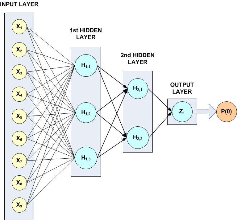
Figure 36, A Binary 3-layer, Classification Network with 7 Inputs and 6 Perceptrons
There are a total of 41 weights in this network. Six are bias weights and the remaining 35 are the weights for the input links to every perceptron, e.g. 35 = 9*3+3*2+2.
Printing is turned on to show progress during the training session.
#include <stdio.h>
#include <imsls.h>
int main(){
float *trainStats;
int i, j, k, m;
int n_patterns =48; /* # of training patterns */
int n_inputs =9; /* 2 nominal (7 classes) and 2 continuous */
int n_nominal =7; /* 2 attributes with 3 and 4 classes each */
int n_continuous =2; /* 2 continuous input attributes */
int n_outputs =1; /* binary classification */
int classification[48];
int nominalAtt[48*7];
int n_cat = 2;
int nomTempIn[48], *nomTempOut, nClass;
float inputData[5*48] =
{
0.00, 0.00, 0, 0, 0, 0.02, 0.02, 0, 1, 0, 0.04, 0.04, 0, 2, 0,
0.06, 0.06, 0, 3, 0, 0.08, 0.08, 1, 0, 0, 0.10, 0.10, 1, 1, 0,
0.12, 0.12, 1, 2, 0, 0.14, 0.14, 1, 3, 0, 0.16, 0.16, 2, 0, 0,
0.18, 0.18, 2, 1, 0, 0.20, 0.20, 2, 2, 0, 0.22, 0.22, 2, 3, 0,
0.24, 0.28, 0, 0, 0, 0.26, 0.30, 0, 1, 0, 0.28, 0.32, 0, 2, 0,
0.30, 0.34, 0, 3, 0, 0.32, 0.36, 1, 0, 0, 0.34, 0.38, 1, 1, 0,
0.36, 0.40, 1, 2, 0, 0.38, 0.42, 1, 3, 0, 0.40, 0.44, 2, 0, 0,
0.42, 0.46, 2, 1, 0, 0.44, 0.48, 2, 2, 0, 0.46, 0.50, 2, 3, 0,
0.52, 0.48, 0, 0, 0, 0.54, 0.50, 0, 1, 1, 0.56, 0.52, 0, 2, 1,
0.58, 0.54, 0, 3, 1, 0.60, 0.56, 1, 0, 1, 0.62, 0.58, 1, 1, 1,
0.64, 0.60, 1, 2, 1, 0.66, 0.62, 1, 3, 1, 0.68, 0.64, 2, 0, 0,
0.70, 0.66, 2, 1, 0, 0.72, 0.68, 2, 2, 0, 0.74, 0.70, 2, 3, 0,
0.76, 0.76, 0, 0, 1, 0.78, 0.78, 0, 1, 1, 0.80, 0.80, 0, 2, 1,
0.82, 0.82, 0, 3, 1, 0.84, 0.84, 1, 0, 1, 0.86, 0.86, 1, 1, 1,
0.88, 0.88, 1, 2, 1, 0.90, 0.90, 1, 3, 1, 0.92, 0.92, 2, 0, 0,
0.94, 0.94, 2, 1, 0, 0.96, 0.96, 2, 2, 0, 0.98, 0.98, 2, 3, 0
};
float contAtt[2*48];
float *classProb;
char *colLabels[] = {"Pattern", "Class=0", "Class=1"};
Imsls_f_NN_Network *network;
printf("\n***********************************\n");
printf("* BINARY CLASSIFICATION EXAMPLE *\n");
printf("***********************************\n\n");
imsls_omp_options(IMSLS_SET_FUNCTIONS_THREAD_SAFE, 1, 0);
/* Setup Continuous Input Attributes and
* Classification Target Arrays
*/
for(i=0; i<n_patterns; i++){
/* Assign input to array for continuous input attributes */
contAtt[2*i] = inputData[i*5];
contAtt[2*i+1] = inputData[i*5+1];
/* Assign input to classification target array*/
classification[i] = (int) inputData[i*5+4];
}
/* Setup Nominal Input Attributes Using Binary Encoding */
m=0;
for(i=0; i<n_cat; i++){
for(j=0; j<n_patterns; j++){
nomTempIn[j] = (int) inputData[j*5+n_continuous+i]+1;
}
nomTempOut = imsls_unsupervised_nominal_filter(n_patterns,
&nClass, nomTempIn, 0);
for(k=0; k<nClass; k++){
for(j=0; j<n_patterns; j++){
nominalAtt[j*n_nominal+m] = nomTempOut[j*nClass+k];
}
m++;
}
imsls_free(nomTempOut);
}
printf("\t TRAINING PATTERNS\n");
printf("\tY N1 N2 Z1 Z2 \n");
for(i=0; i<n_patterns; i++){
j = (int) inputData[i*5+2];
k = (int) inputData[i*5+3];
printf("\t%d %d %d %g %g \n", classification[i], j, k,
contAtt[i*2], contAtt[i*2+1]);
}
printf("\n");
network = imsls_f_mlff_network_init(n_inputs, n_outputs);
imsls_f_mlff_network(network,
IMSLS_CREATE_HIDDEN_LAYER, 3,
0);
imsls_f_mlff_network(network,
IMSLS_CREATE_HIDDEN_LAYER, 2,
IMSLS_LINK_ALL,
0);
/* Note the following statement is for repeatable output */
imsls_random_seed_set(5555);
/* Train Classification Network */
printf("STARTING NETWORK TRAINING\n");
trainStats = imsls_f_mlff_classification_trainer (network,
n_patterns, n_nominal, n_continuous, classification,
nominalAtt, contAtt,
IMSLS_PRINT,
IMSLS_PREDICTED_CLASS_PROB, &classProb,
0);
/* Print class predictions*/
imsls_f_write_matrix("Predicted Classification Probabilities",
n_patterns, n_outputs , classProb,
IMSLS_ROW_NUMBER,
IMSLS_COL_LABELS, colLabels,
0);
}
Output
Notice that although by default the maximum number of epoch iterations in Stage I training is 15, in this case Stage I optimization is halted after the first epoch. This occurs because the minimum entropy for that epoch is less than the default tolerance.
***********************************
* BINARY CLASSIFICATION EXAMPLE *
***********************************
TRAINING PATTERNS
Y N1 N2 Z1 Z2
0 0 0 0 0
0 0 1 0.02 0.02
0 0 2 0.04 0.04
0 0 3 0.06 0.06
0 1 0 0.08 0.08
0 1 1 0.1 0.1
0 1 2 0.12 0.12
0 1 3 0.14 0.14
0 2 0 0.16 0.16
0 2 1 0.18 0.18
0 2 2 0.2 0.2
0 2 3 0.22 0.22
0 0 0 0.24 0.28
0 0 1 0.26 0.3
0 0 2 0.28 0.32
0 0 3 0.3 0.34
0 1 0 0.32 0.36
0 1 1 0.34 0.38
0 1 2 0.36 0.4
0 1 3 0.38 0.42
0 2 0 0.4 0.44
0 2 1 0.42 0.46
0 2 2 0.44 0.48
0 2 3 0.46 0.5
0 0 0 0.52 0.48
1 0 1 0.54 0.5
1 0 2 0.56 0.52
1 0 3 0.58 0.54
1 1 0 0.6 0.56
1 1 1 0.62 0.58
1 1 2 0.64 0.6
1 1 3 0.66 0.62
0 2 0 0.68 0.64
0 2 1 0.7 0.66
0 2 2 0.72 0.68
0 2 3 0.74 0.7
1 0 0 0.76 0.76
1 0 1 0.78 0.78
1 0 2 0.8 0.8
1 0 3 0.82 0.82
1 1 0 0.84 0.84
1 1 1 0.86 0.86
1 1 2 0.88 0.88
1 1 3 0.9 0.9
0 2 0 0.92 0.92
0 2 1 0.94 0.94
0 2 2 0.96 0.96
0 2 3 0.98 0.98
STARTING NETWORK TRAINING
TRAINING PARAMETERS:
Stage II Opt. = 1
n_epochs = 15
epoch_size = 48
maxIterations = 1000
maxFunctionEval = 1000
maxStep = 10.000000
functionTol = 2.42218e-005
gradientTol = 0.000345267
accuracy = 0.000345267
n_inputs = 9
n_continuous = 2
n_nominal = 7
n_classes = 2
n_outputs = 1
n_patterns = 48
n_layers = 3
n_perceptrons = 6
n_weights = 41
STAGE I TRAINING STARTING
Stage I: Epoch 1 - Cross-Entropy Error = 1.03973e-005 (Iterations=58)
(CPU Min.=0.000260)
Stage I Training Converged at Epoch = 1
STAGE I FINAL CROSS-ENTROPY ERROR = 0.000010 (CPU Min.=0.000260)
OPTIMUM WEIGHTS AFTER STAGE I TRAINING:
weight[0] = -0.634574 weight[1] = 3.10432
weight[2] = 0.753153 weight[3] = 3.26621
weight[4] = 0.873874 weight[5] = 0.564623
weight[6] = 0.574684 weight[7] = 2.03545
weight[8] = 2.11041 weight[9] = 4.53693
weight[10] = 3.17946 weight[11] = -10.908
weight[12] = -1.12353 weight[13] = 0.915452
weight[14] = -0.737025 weight[15] = -0.44498
weight[16] = 11.1242 weight[17] = 8.99682
weight[18] = 2.17726 weight[19] = 1.82712
weight[20] = -8.49784 weight[21] = -3.14366
weight[22] = -0.0180527 weight[23] = 0.618158
weight[24] = -0.243258 weight[25] = 13.5949
weight[26] = 11.9534 weight[27] = -4.83385
weight[28] = -18.9217 weight[29] = -9.0807
weight[30] = -7.01863 weight[31] = -15.0597
weight[32] = -17.7305 weight[33] = 23.6268
weight[34] = 11.2716 weight[35] = -6.76151
weight[36] = -13.0134 weight[37] = -14.1513
weight[38] = 17.8283 weight[39] = 21.7138
weight[40] = -19.8484
STAGE I TRAINING CONVERGED
STAGE I CROSS-ENTROPY ERROR = 0.000010
0 PATTERNS OUT OF 48 INCORRECTLY CLASSIFIED
GRADIENT AT THE OPTIMUM WEIGHTS
-->g[0] = 0.000000 weight[0] = -0.634574
-->g[1] = -0.000001 weight[1] = 3.104319
-->g[2] = 0.000000 weight[2] = 0.753153
-->g[3] = -0.000001 weight[3] = 3.266206
-->g[4] = 0.000000 weight[4] = 0.873874
-->g[5] = 0.000000 weight[5] = 0.564623
-->g[6] = 0.000000 weight[6] = 0.574684
-->g[7] = -0.000000 weight[7] = 2.035449
-->g[8] = -0.000000 weight[8] = 2.110413
-->g[9] = 0.000000 weight[9] = 4.536931
-->g[10] = -0.000005 weight[10] = 3.179461
-->g[11] = 0.000000 weight[11] = -10.908046
-->g[12] = -0.000005 weight[12] = -1.123529
-->g[13] = 0.000000 weight[13] = 0.915452
-->g[14] = 0.000000 weight[14] = -0.737025
-->g[15] = 0.000000 weight[15] = -0.444980
-->g[16] = -0.000003 weight[16] = 11.124193
-->g[17] = -0.000003 weight[17] = 8.996821
-->g[18] = 0.000000 weight[18] = 2.177265
-->g[19] = -0.000004 weight[19] = 1.827117
-->g[20] = 0.000000 weight[20] = -8.497839
-->g[21] = -0.000004 weight[21] = -3.143664
-->g[22] = 0.000000 weight[22] = -0.018053
-->g[23] = 0.000000 weight[23] = 0.618158
-->g[24] = 0.000000 weight[24] = -0.243258
-->g[25] = -0.000002 weight[25] = 13.594892
-->g[26] = -0.000002 weight[26] = 11.953360
-->g[27] = 0.000001 weight[27] = -4.833848
-->g[28] = 0.000000 weight[28] = -18.921690
-->g[29] = 0.000000 weight[29] = -9.080699
-->g[30] = 0.000001 weight[30] = -7.018632
-->g[31] = 0.000001 weight[31] = -15.059658
-->g[32] = 0.000000 weight[32] = -17.730463
-->g[33] = -0.000010 weight[33] = 23.626806
-->g[34] = -0.000010 weight[34] = 11.271611
-->g[35] = -0.000001 weight[35] = -6.761511
-->g[36] = -0.000005 weight[36] = -13.013445
-->g[37] = -0.000004 weight[37] = -14.151301
-->g[38] = 0.000001 weight[38] = 17.828314
-->g[39] = 0.000001 weight[39] = 21.713770
-->g[40] = -0.000010 weight[40] = -19.848421
Training Completed - leaving training engine (CPU Min.=0.000260)
Predicted Classification Probabilities
Pattern Class=0
1 1
2 1
3 1
4 1
5 1
6 1
7 1
8 1
9 1
10 1
11 1
12 1
13 1
14 1
15 1
16 1
17 1
18 1
19 1
20 1
21 1
22 1
23 1
24 1
25 1
26 0
27 0
28 0
29 0
30 0
31 0
32 0
33 1
34 1
35 1
36 1
37 0
38 0
39 0
40 0
41 0
42 0
43 0
44 0
45 1
46 1
47 1
48 1
Example 2
Fisher’s (1936) Iris data is often used for benchmarking discriminant analysis and classification solutions. It is part of the IMSL data sets and consists of the following continuous input attributes and classification target:
Continuous Attributes – X1(sepal length), X2(sepal width), X3(petal length), and X4(petal width)
Classification Target (Iris Type) – Setosa, Versicolour or Virginica.
These data consist of 150 patterns. Since all pattern input attributes are continuous, linear discriminant analysis can be used for classifying these patterns, see Example 1 of imsls_f_discriminant_analysis. Linear discriminant analysis is able to correctly classify 98% of the training patterns. In this example, the simple neural network illustrated in the following figure is able to achieve 100% accuracy.
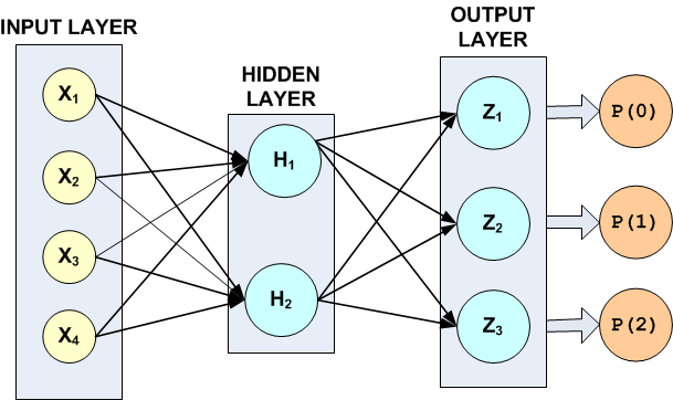
Figure 37, A 2-layer, Classification Network with 4 Inputs 5 Perceptrons and a Target Classification with 3 Classes
The hidden layer in this example consists of only two perceptrons with logistic activation. Since the target attribute in this example has three classes, the network output layer consists of three perceptrons, one for each class.
There are a total of 19 weights in this network. Fourteen of the weights are assigned to the input links, i.e., 4 × 2 + 2 × 3 = 14. The last five weights are the bias weights for each of the five network perceptrons. All weights were initialized using principal components, i.e. method = IMSLS_PRINCIPAL_COMPONENTS.
Although in these data the continuous attributes have similar ranges, they were scaled using z‑score scaling to make network training more efficient. For more details, see imsls_f_scale_filter.
For non-binary classification problems, imsls_f_mlff_classification_trainer uses softmax activation for output perceptrons. This ensures that the estimates of the classification probabilities sum to one, i.e.
Note that the default setting for IMSLS_MAX_STEP was changed from 10 to 1000. The default setting converged to a network with 100% classification accuracy. However, the following warning message appeared:
*** WARNING Error IMSLS_UNBOUNDED from imsls_d_mlff_classification_trainer.
*** Five consecutive steps of length "max_step" have been taken;
*** either the function is unbounded below, or has a finite
*** asymptote in some direction or the maximum allowable step size
*** "max_step" is too small.
In addition, the number of iterations used for each epoch were well below the default maximum (1000), and the gradients at the optimum solution for this network were not zero.
STAGE I TRAINING STARTING
Stage I: Epoch 1 - Cross-Entropy Error = 5.50552 (Iterations=40) (CPU Min.=0.000260)
Stage I: Epoch 2 - Cross-Entropy Error = 5.65875 (Iterations=69) (CPU Min.=0.000260)
Stage I: Epoch 3 - Cross-Entropy Error = 4.83886 (Iterations=81) (CPU Min.=0.000260)
Stage I: Epoch 4 - Cross-Entropy Error = 5.94979 (Iterations=108) (CPU Min.=0.000521)
Stage I: Epoch 5 - Cross-Entropy Error = 5.54461 (Iterations=47) (CPU Min.=0.000260)
Stage I: Epoch 6 - Cross-Entropy Error = 6.04163 (Iterations=51) (CPU Min.=0.000260)
Stage I: Epoch 7 - Cross-Entropy Error = 5.95148 (Iterations=151) (CPU Min.=0.000521)
Stage I: Epoch 8 - Cross-Entropy Error = 5.5646 (Iterations=55) (CPU Min.=0.000260)
Stage I: Epoch 9 - Cross-Entropy Error = 5.94914 (Iterations=442) (CPU Min.=0.001563)
Stage I: Epoch 10 - Cross-Entropy Error = 5.94381 (Iterations=271) (CPU Min.=0.001302)
Stage I: Epoch 11 - Cross-Entropy Error = 5.41955 (Iterations=35) (CPU Min.=0.000000)
Stage I: Epoch 12 - Cross-Entropy Error = 6.01766 (Iterations=48) (CPU Min.=0.000260)
Stage I: Epoch 13 - Cross-Entropy Error = 4.20551 (Iterations=112) (CPU Min.=0.000521)
Stage I: Epoch 14 - Cross-Entropy Error = 5.95085 (Iterations=103) (CPU Min.=0.000260)
Stage I: Epoch 15 - Cross-Entropy Error = 5.9596 (Iterations=55) (CPU Min.=0.000260)
Stage I: Epoch 16 - Cross-Entropy Error = 5.96131 (Iterations=59) (CPU Min.=0.000260)
Stage I: Epoch 17 - Cross-Entropy Error = 4.83231 (Iterations=74) (CPU Min.=0.000260)
Stage I: Epoch 18 - Cross-Entropy Error = 17.1345 (Iterations=30) (CPU Min.=0.000260)
Stage I: Epoch 19 - Cross-Entropy Error = 5.95569 (Iterations=92) (CPU Min.=0.000260)
Stage I: Epoch 20 - Cross-Entropy Error = 3.15336 (Iterations=46) (CPU Min.=0.000260)
GRADIENT AT THE OPTIMUM WEIGHTS
-->g[0] = 0.675632 weight[0] = 0.075861
-->g[1] = -0.953480 weight[1] = -0.078585
-->g[2] = 1.065184 weight[2] = 2.841074
-->g[3] = 0.535531 weight[3] = -0.941049
-->g[4] = -0.019011 weight[4] = -10.638772
-->g[5] = 0.001459 weight[5] = -14.573394
-->g[6] = -0.031098 weight[6] = 6.037813
-->g[7] = -0.035305 weight[7] = 72.382073
-->g[8] = 0.011015 weight[8] = -73.564433
-->g[9] = 0.000000 weight[9] = -14.853988
-->g[10] = -0.074332 weight[10] = 2.057743
-->g[11] = 0.000522 weight[11] = -39.952435
-->g[12] = 0.063316 weight[12] = 73.164141
-->g[13] = -0.000522 weight[13] = 57.065975
-->g[14] = 1.279914 weight[14] = -0.661036
-->g[15] = -0.043097 weight[15] = -61.171894
-->g[16] = 0.003227 weight[16] = 24.236722
-->g[17] = -0.108146 weight[17] = 14.968424
-->g[18] = 0.104919 weight[18] = -39.079343
Combined, this information suggests that either the default tolerances were too high or the maximum step size was too small. As shown in the output below, when the maximum step size was changed to 1000, the number of iterations increased, the gradients went to zero and the warning message for step size disappeared.
#include <stdio.h>
#include <imsls.h>
/* ********************************************************************
* Two Layer Feed-Forward Network with 4 inputs, all
* continuous, and 3 classification categories.
*
* This is a well known database to be found in the pattern
* recognition literature. Fisher's paper is often cited.
* The data set contains 3 classes of 50 instances each,
* where each class refers to a type of iris plant. One class is
* linearly separable from the other 2; the latter are NOT linearly
* separable from each other.
*
* Predicted attribute: class of iris plant.
* 1=Iris Setosa, 2=Iris Versicolour, and 3=Iris Virginica
*
* Input Attributes (4 Continuous Attributes)
* X1: Sepal length,
* X2: Sepal width,
* X3: Petal length,
* and X4: Petal width
*
*********************************************************************/
int main(){
float *predicted_class_prob, *class_error, *trainStats;
int i, j;
int n_patterns = 150;
int n_inputs = 4; /* all continuous inputs*/
int n_nominal = 0; /* no nominal */
int n_continuous = 4;
int n_outputs = 3;
int *nominalAtt=NULL;
int *predicted_class;
int act_fcn[3] = {1, 1, 1};
int classification[150];
float unscaledX[150], scaledX[150];
float contAtt[4*150];
float *irisData;
float mean[4], s[4], center, spread;
double startTime, endTime;
char *colLabels[] = {"Pattern", "Class=0", "Class=1", "Class=2"};
char prtLabel[] =
"Predicted_Class | P(0) P(1) P(2) | Class_Error";
char dashes[] =
"-------------------------------------------------------------";
char *filename = "iris_classification.txt";
/* Declare mlff network structure */
Imsls_f_NN_Network *network;
printf("*******************************************************\n");
printf("* IRIS CLASSIFICATION EXAMPLE *\n");
printf("*******************************************************\n");
imsls_omp_options(IMSLS_SET_FUNCTIONS_THREAD_SAFE, 1, 0);
/*
* irisData[]: The raw data matrix. This is a 2-D matrix with 150
* rows and 5 columns. The last 4 columns are the
* continuous input attributes and the 1st column is
* the classification category (1-3). These data
* contain no nominal input attributes.
*/
irisData = imsls_f_data_sets(3,0);
/*
* Setup the continuous attribute input array, contAtt[], and the
* network target classification array, classification[], using the
* above raw data matrix.
*/
for(i=0; i < n_patterns; i++){
classification[i] = (int)irisData[i*5]-1;
for(j=1; j<5; j++){
contAtt[i*4+j-1] = irisData[i*5+j];
}
}
/* Scale continuous input attributes using z-score method */
for(j=0; j<n_continuous; j++){
for(i=0; i<n_patterns; i++)
unscaledX[i] = contAtt[i*n_continuous+j];
imsls_f_scale_filter(n_patterns, unscaledX, 2,
IMSLS_RETURN_USER, scaledX,
IMSLS_RETURN_CENTER_SPREAD, ¢er, &spread, 0);
for(i=0; i<n_patterns; i++)
contAtt[i*n_continuous+j] = scaledX[i];
mean[j] = center;
s[j] = spread;
}
printf("Scale Parameters: \n");
for(j=0; j<n_continuous; j++){
printf("Var %d Mean = %f S = %f \n",j+1, mean[j], s[j]);
}
network = imsls_f_mlff_network_init(n_inputs, n_outputs);
imsls_f_mlff_network(network, IMSLS_CREATE_HIDDEN_LAYER, 2,
IMSLS_LINK_ALL, 0);
/* Note the following statement is for repeatable output */
imsls_random_seed_set(5555);
/* Train Classification Network */
startTime = imsls_ctime();
trainStats = imsls_f_mlff_classification_trainer (network,
n_patterns,
n_nominal,
n_continuous,
classification,
nominalAtt,
contAtt,
IMSLS_PRINT,
IMSLS_STAGE_I, 20, 150,
IMSLS_WEIGHT_INITIALIZATION_METHOD, IMSLS_PRINCIPAL_COMPONENTS,
IMSLS_MAX_STEP, 1000.0,
IMSLS_PREDICTED_CLASS, &predicted_class,
IMSLS_PREDICTED_CLASS_PROB, &predicted_class_prob,
IMSLS_CLASS_ERROR, &class_error,
0);
endTime = imsls_ctime();
printf("%s\n", dashes);
printf("Minimum Cross-Entropy Error: %g\n", trainStats[0]);
printf("Classification Error Rate: %f\n", trainStats[5]);
printf("Execution Time (Sec.): %f\n\n", (endTime-startTime));
printf("%s\n",prtLabel);
printf("%s\n",dashes);
for(i=0; i<n_patterns; i++){
printf(" %d ", predicted_class[i]);
printf(" | %f %f %f | %f\n", predicted_class_prob[i*3],
predicted_class_prob[i*3+1], predicted_class_prob[i*3+2],
class_error[i]);
if(i==49 || i==99){
printf("%s\n",prtLabel);
printf("%s\n",dashes);
}
}
imsls_f_mlff_network_write(network, filename, IMSLS_PRINT, 0);
}
Output
Note that the misclassification error rate is zero and Stage I training halts automatically at the 16th epoch because the cross-entropy error after the 16th epoch is below the default tolerance.
*******************************************************
* IRIS CLASSIFICATION EXAMPLE *
*******************************************************
Scale Parameters:
Var 1 Mean = 5.843334 S = 0.828065
Var 2 Mean = 3.057333 S = 0.435866
Var 3 Mean = 3.758000 S = 1.765298
Var 4 Mean = 1.199333 S = 0.762238
TRAINING PARAMETERS:
Stage II Opt. = 1
n_epochs = 20
epoch_size = 150
maxIterations = 1000
maxFunctionEval = 1000
maxStep = 1000.000000
functionTol = 2.42218e-005
gradientTol = 0.000345267
accuracy = 0.000345267
n_inputs = 4
n_continuous = 4
n_nominal = 0
n_classes = 3
n_outputs = 3
n_patterns = 150
n_layers = 2
n_perceptrons = 5
n_weights = 19
STAGE I TRAINING STARTING
Stage I: Epoch 1 - Cross-Entropy Error = 4.92197 (Iterations=77)
(CPU Min.=0.000260)
Stage I: Epoch 2 - Cross-Entropy Error = 5.95334 (Iterations=234)
(CPU Min.=0.001042)
Stage I: Epoch 3 - Cross-Entropy Error = 5.95312 (Iterations=237)
(CPU Min.=0.000781)
Stage I: Epoch 4 - Cross-Entropy Error = 74.9249 (Iterations=30)
(CPU Min.=0.000260)
Stage I: Epoch 5 - Cross-Entropy Error = 4.92196 (Iterations=130)
(CPU Min.=0.000260)
Stage I: Epoch 6 - Cross-Entropy Error = 5.9565 (Iterations=208)
(CPU Min.=0.000781)
Stage I: Epoch 7 - Cross-Entropy Error = 4.92199 (Iterations=99)
(CPU Min.=0.000521)
Stage I: Epoch 8 - Cross-Entropy Error = 4.92197 (Iterations=117)
(CPU Min.=0.000260)
Stage I: Epoch 9 - Cross-Entropy Error = 5.06757 (Iterations=500)
(CPU Min.=0.001302)
Stage I: Epoch 10 - Cross-Entropy Error = 5.94276 (Iterations=136)
(CPU Min.=0.000260)
Stage I: Epoch 11 - Cross-Entropy Error = 4.92198 (Iterations=80)
(CPU Min.=0.000260)
Stage I: Epoch 12 - Cross-Entropy Error = 4.92199 (Iterations=100)
(CPU Min.=0.000260)
Stage I: Epoch 13 - Cross-Entropy Error = 4.92199 (Iterations=87)
(CPU Min.=0.000260)
Stage I: Epoch 14 - Cross-Entropy Error = 5.95085 (Iterations=245)
(CPU Min.=0.000781)
Stage I: Epoch 15 - Cross-Entropy Error = 5.95099 (Iterations=165)
(CPU Min.=0.001042)
Stage I: Epoch 16 - Cross-Entropy Error = 2.5034e-005 (Iterations=134)
(CPU Min.=0.000521)
Stage I Training Converged at Epoch = 16
STAGE I FINAL CROSS-ENTROPY ERROR = 0.000025 (CPU Min.=0.008854)
OPTIMUM WEIGHTS AFTER STAGE I TRAINING:
weight[0] = 0.3079 weight[1] = -0.12877
weight[2] = 4.51303 weight[3] = -1.90144
weight[4] = -14.3699 weight[5] = -519.855
weight[6] = 1317.12 weight[7] = 2756.14
weight[8] = -3454.11 weight[9] = -193.738
weight[10] = 116.785 weight[11] = -1310.03
weight[12] = 3339.35 weight[13] = 1505.56
weight[14] = 1.01363 weight[15] = -3010.6
weight[16] = 1785.05 weight[17] = 682.292
weight[18] = -2467.38
STAGE I TRAINING CONVERGED
STAGE I CROSS-ENTROPY ERROR = 0.000025
0 PATTERNS OUT OF 150 INCORRECTLY CLASSIFIED
GRADIENT AT THE OPTIMUM WEIGHTS
-->g[0] = 0.001389 weight[0] = 0.307900
-->g[1] = 0.001205 weight[1] = -0.128770
-->g[2] = 0.000713 weight[2] = 4.513030
-->g[3] = 0.000269 weight[3] = -1.901438
-->g[4] = 0.000000 weight[4] = -14.369907
-->g[5] = 0.000000 weight[5] = -519.854919
-->g[6] = 0.000000 weight[6] = 1317.116821
-->g[7] = 0.000000 weight[7] = 2756.140625
-->g[8] = 0.000000 weight[8] = -3454.105713
-->g[9] = 0.000000 weight[9] = -193.738205
-->g[10] = -0.000002 weight[10] = 116.785263
-->g[11] = 0.000000 weight[11] = -1310.028076
-->g[12] = 0.000002 weight[12] = 3339.346680
-->g[13] = 0.000000 weight[13] = 1505.561646
-->g[14] = -0.000807 weight[14] = 1.013626
-->g[15] = 0.000000 weight[15] = -3010.596680
-->g[16] = 0.000002 weight[16] = 1785.052979
-->g[17] = -0.000003 weight[17] = 682.292419
-->g[18] = 0.000002 weight[18] = -2467.379395
Training Completed - leaving training engine (CPU Min.=0.008854)
-------------------------------------------------------------
Minimum Cross-Entropy Error: 2.5034e-005
Classification Error Rate: 0.000000
Execution Time (Sec.): 0.531250
Predicted_Class | P(0) P(1) P(2) | Class_Error
-------------------------------------------------------------
0 | 1.000000 0.000000 0.000000 | 0.000000
0 | 1.000000 0.000000 0.000000 | 0.000000
0 | 1.000000 0.000000 0.000000 | 0.000000
0 | 1.000000 0.000000 0.000000 | 0.000000
0 | 1.000000 0.000000 0.000000 | 0.000000
0 | 1.000000 0.000000 0.000000 | 0.000000
0 | 1.000000 0.000000 0.000000 | 0.000000
0 | 1.000000 0.000000 0.000000 | 0.000000
0 | 1.000000 0.000000 0.000000 | 0.000000
0 | 1.000000 0.000000 0.000000 | 0.000000
0 | 1.000000 0.000000 0.000000 | 0.000000
0 | 1.000000 0.000000 0.000000 | 0.000000
0 | 1.000000 0.000000 0.000000 | 0.000000
0 | 1.000000 0.000000 0.000000 | 0.000000
0 | 1.000000 0.000000 0.000000 | 0.000000
0 | 1.000000 0.000000 0.000000 | 0.000000
0 | 1.000000 0.000000 0.000000 | 0.000000
0 | 1.000000 0.000000 0.000000 | 0.000000
0 | 1.000000 0.000000 0.000000 | 0.000000
0 | 1.000000 0.000000 0.000000 | 0.000000
0 | 1.000000 0.000000 0.000000 | 0.000000
0 | 1.000000 0.000000 0.000000 | 0.000000
0 | 1.000000 0.000000 0.000000 | 0.000000
0 | 1.000000 0.000000 0.000000 | 0.000000
0 | 1.000000 0.000000 0.000000 | 0.000000
0 | 1.000000 0.000000 0.000000 | 0.000000
0 | 1.000000 0.000000 0.000000 | 0.000000
0 | 1.000000 0.000000 0.000000 | 0.000000
0 | 1.000000 0.000000 0.000000 | 0.000000
0 | 1.000000 0.000000 0.000000 | 0.000000
0 | 1.000000 0.000000 0.000000 | 0.000000
0 | 1.000000 0.000000 0.000000 | 0.000000
0 | 1.000000 0.000000 0.000000 | 0.000000
0 | 1.000000 0.000000 0.000000 | 0.000000
0 | 1.000000 0.000000 0.000000 | 0.000000
0 | 1.000000 0.000000 0.000000 | 0.000000
0 | 1.000000 0.000000 0.000000 | 0.000000
0 | 1.000000 0.000000 0.000000 | 0.000000
0 | 1.000000 0.000000 0.000000 | 0.000000
0 | 1.000000 0.000000 0.000000 | 0.000000
0 | 1.000000 0.000000 0.000000 | 0.000000
0 | 1.000000 0.000000 0.000000 | 0.000000
0 | 1.000000 0.000000 0.000000 | 0.000000
0 | 1.000000 0.000000 0.000000 | 0.000000
0 | 1.000000 0.000000 0.000000 | 0.000000
0 | 1.000000 0.000000 0.000000 | 0.000000
0 | 1.000000 0.000000 0.000000 | 0.000000
0 | 1.000000 0.000000 0.000000 | 0.000000
0 | 1.000000 0.000000 0.000000 | 0.000000
0 | 1.000000 0.000000 0.000000 | 0.000000
Predicted_Class | P(0) P(1) P(2) | Class_Error
-------------------------------------------------------------
1 | 0.000000 1.000000 0.000000 | 0.000000
1 | 0.000000 1.000000 0.000000 | 0.000000
1 | 0.000000 1.000000 0.000000 | 0.000000
1 | 0.000000 1.000000 0.000000 | 0.000000
1 | 0.000000 1.000000 0.000000 | 0.000000
1 | 0.000000 1.000000 0.000000 | 0.000000
1 | 0.000000 1.000000 0.000000 | 0.000000
1 | 0.000000 1.000000 0.000000 | 0.000000
1 | 0.000000 1.000000 0.000000 | 0.000000
1 | 0.000000 1.000000 0.000000 | 0.000000
1 | 0.000000 1.000000 0.000000 | 0.000000
1 | 0.000000 1.000000 0.000000 | 0.000000
1 | 0.000000 1.000000 0.000000 | 0.000000
1 | 0.000000 1.000000 0.000000 | 0.000000
1 | 0.000000 1.000000 0.000000 | 0.000000
1 | 0.000000 1.000000 0.000000 | 0.000000
1 | 0.000000 1.000000 0.000000 | 0.000000
1 | 0.000000 1.000000 0.000000 | 0.000000
1 | 0.000000 1.000000 0.000000 | 0.000000
1 | 0.000000 1.000000 0.000000 | 0.000000
1 | 0.000000 1.000000 0.000000 | 0.000000
1 | 0.000000 1.000000 0.000000 | 0.000000
1 | 0.000000 1.000000 0.000000 | 0.000000
1 | 0.000000 0.999999 0.000001 | 0.000001
1 | 0.000000 1.000000 0.000000 | 0.000000
1 | 0.000000 1.000000 0.000000 | 0.000000
1 | 0.000000 0.999994 0.000006 | 0.000006
1 | 0.000000 1.000000 0.000000 | 0.000000
1 | 0.000000 1.000000 0.000000 | 0.000000
1 | 0.000000 1.000000 0.000000 | 0.000000
1 | 0.000000 1.000000 0.000000 | 0.000000
1 | 0.000000 1.000000 0.000000 | 0.000000
1 | 0.000000 1.000000 0.000000 | 0.000000
1 | 0.000000 0.999994 0.000006 | 0.000006
1 | 0.000000 1.000000 0.000000 | 0.000000
1 | 0.000000 1.000000 0.000000 | 0.000000
1 | 0.000000 1.000000 0.000000 | 0.000000
1 | 0.000000 1.000000 0.000000 | 0.000000
1 | 0.000000 1.000000 0.000000 | 0.000000
1 | 0.000000 1.000000 0.000000 | 0.000000
1 | 0.000000 1.000000 0.000000 | 0.000000
1 | 0.000000 1.000000 0.000000 | 0.000000
1 | 0.000000 1.000000 0.000000 | 0.000000
1 | 0.000000 1.000000 0.000000 | 0.000000
1 | 0.000000 1.000000 0.000000 | 0.000000
1 | 0.000000 1.000000 0.000000 | 0.000000
1 | 0.000000 1.000000 0.000000 | 0.000000
1 | 0.000000 1.000000 0.000000 | 0.000000
1 | 0.000002 0.999998 0.000000 | 0.000002
1 | 0.000000 1.000000 0.000000 | 0.000000
Predicted_Class | P(0) P(1) P(2) | Class_Error
-------------------------------------------------------------
2 | 0.000000 0.000000 1.000000 | 0.000000
2 | 0.000000 0.000000 1.000000 | 0.000000
2 | 0.000000 0.000000 1.000000 | 0.000000
2 | 0.000000 0.000000 1.000000 | 0.000000
2 | 0.000000 0.000000 1.000000 | 0.000000
2 | 0.000000 0.000000 1.000000 | 0.000000
2 | 0.000000 0.000000 1.000000 | 0.000000
2 | 0.000000 0.000000 1.000000 | 0.000000
2 | 0.000000 0.000000 1.000000 | 0.000000
2 | 0.000000 0.000000 1.000000 | 0.000000
2 | 0.000000 0.000000 1.000000 | 0.000000
2 | 0.000000 0.000000 1.000000 | 0.000000
2 | 0.000000 0.000000 1.000000 | 0.000000
2 | 0.000000 0.000000 1.000000 | 0.000000
2 | 0.000000 0.000000 1.000000 | 0.000000
2 | 0.000000 0.000000 1.000000 | 0.000000
2 | 0.000000 0.000000 1.000000 | 0.000000
2 | 0.000000 0.000000 1.000000 | 0.000000
2 | 0.000000 0.000000 1.000000 | 0.000000
2 | 0.000000 0.000000 1.000000 | 0.000000
2 | 0.000000 0.000000 1.000000 | 0.000000
2 | 0.000000 0.000000 1.000000 | 0.000000
2 | 0.000000 0.000000 1.000000 | 0.000000
2 | 0.000000 0.000000 1.000000 | 0.000000
2 | 0.000000 0.000000 1.000000 | 0.000000
2 | 0.000000 0.000000 1.000000 | 0.000000
2 | 0.000000 0.000000 1.000000 | 0.000000
2 | 0.000000 0.000000 1.000000 | 0.000000
2 | 0.000000 0.000000 1.000000 | 0.000000
2 | 0.000000 0.000000 1.000000 | 0.000000
2 | 0.000000 0.000000 1.000000 | 0.000000
2 | 0.000000 0.000000 1.000000 | 0.000000
2 | 0.000000 0.000000 1.000000 | 0.000000
2 | 0.000000 0.000011 0.999989 | 0.000011
2 | 0.000000 0.000000 1.000000 | 0.000000
2 | 0.000000 0.000000 1.000000 | 0.000000
2 | 0.000000 0.000000 1.000000 | 0.000000
2 | 0.000000 0.000000 1.000000 | 0.000000
2 | 0.000000 0.000000 1.000000 | 0.000000
2 | 0.000000 0.000000 1.000000 | 0.000000
2 | 0.000000 0.000000 1.000000 | 0.000000
2 | 0.000000 0.000000 1.000000 | 0.000000
2 | 0.000000 0.000000 1.000000 | 0.000000
2 | 0.000000 0.000000 1.000000 | 0.000000
2 | 0.000000 0.000000 1.000000 | 0.000000
2 | 0.000000 0.000000 1.000000 | 0.000000
2 | 0.000000 0.000000 1.000000 | 0.000000
2 | 0.000000 0.000000 1.000000 | 0.000000
2 | 0.000000 0.000000 1.000000 | 0.000000
2 | 0.000000 0.000000 1.000000 | 0.000000
Opening iris_classification.txt for writing network data structure
Writing Neural Network... 55 Lines written to network file.
File iris_classification.txt closed.


