Usage Notes
Unconstrained Minimization
The unconstrained minimization problem can be stated as follows:
where f : Rn→ R is at least continuous. The routines for unconstrained minimization are grouped into three categories: univariate functions (UV***), multivariate functions (UM***), and nonlinear least squares (UNLS*).
For the univariate function routines, it is assumed that the function is unimodal within the specified interval. Otherwise, only a local minimum can be expected. For further discussion on unimodality, see Brent (1973).
A quasi-Newton method is used for the multivariate function routines UMINF and UMING, whereas UMIDH and UMIAH use a modified Newton algorithm. The routines UMCGF and UMCGG make use of a conjugate gradient approach, and UMPOL uses a polytope method. For more details on these algorithms, see the documentation for the corresponding routines.
The nonlinear least squares routines use a modified Levenberg-Marquardt algorithm. If the nonlinear least squares problem is a nonlinear data-fitting problem, then software that is designed to deliver better statistical output may be useful; see IMSL (1991).
These routines are designed to find only a local minimum point. However, a function may have many local minima. It is often possible to obtain a better local solution by trying different initial points and intervals.
High precision arithmetic is recommended for the routines that use only function values. Also it is advised that the derivative-checking routines CH*** be used to ensure the accuracy of the user-supplied derivative evaluation subroutines.
Minimization with Simple Bounds
The minimization with simple bounds problem can be stated as follows:
where f : Rn→ R, and all the variables are not necessarily bounded.
The routines BCO** use the same algorithms as the routines UMI**, and the routines BCLS* are the corresponding routines of UNLS*. The only difference is that an active set strategy is used to ensure that each variable stays within its bounds. The routine BCPOL uses a function comparison method similar to the one used by UMPOL. Convergence for these polytope methods is not guaranteed; therefore, these routines should be used as a last alternative.
Linearly Constrained Minimization
The linearly constrained minimization problem can be stated as follows:
where f : Rn→ R, A is an m ´ n coefficient matrix, and b is a vector of length m. If f(x) is linear, then the problem is a linear programming problem; if f(x) is quadratic, the problem is a quadratic programming problem.
The routine DLPRS uses an active set strategy to solve small- to medium-sized linear programming problems. No sparsity is assumed since the coefficients are stored in full matrix form.
The routine QPROG is designed to solve convex quadratic programming problems using a dual quadratic programming algorithm. If the given Hessian is not positive definite, then QPROG modifies it to be positive definite. In this case, output should be interpreted with care.
The routines LCONF and LCONG use an iterative method to solve the linearly constrained problem with a general objective function. For a detailed description of the algorithm, see Powell (1988, 1989).
Nonlinearly Constrained Minimization
The nonlinearly constrained minimization problem can be stated as follows:
where f : Rn→ R and gi : R→ R, for i = 1, 2, …, m
The routines NNLPF and NNLPG use a sequential equality constrained quadratic programming method. A more complete discussion of this algorithm can be found in the documentation.
Selection of Routines
The following general guidelines are provided to aid in the selection of the appropriate routine.
Unconstrained Minimization
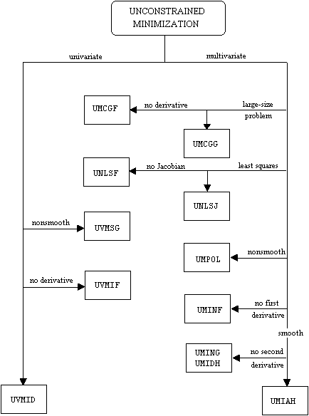
1. For the univariate case, use UVMID when the gradient is available, and use UVMIF when it is not. If discontinuities exist, then use UVMGS.
2. For the multivariate case, use UMCG* when storage is a problem, and use UMPOL when the function is nonsmooth. Otherwise, use UMI** depending on the availability of the gradient and the Hessian.
3. For least squares problems, use UNLSJ when the Jacobian is available, and use UNLSF when it is not.
Minimization with Simple Bounds
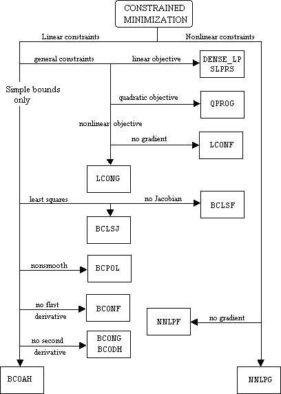
1. Use BCONF when only function values are available. When first derivatives are available, use either BCONG or BCODH. If first and second derivatives are available, then use BCOAH.
2. For least squares, use BCLSF or BCLSJ depending on the availability of the Jacobian.
3. Use BCPOL for nonsmooth functions that could not be solved satisfactorily by the other routines.
The following charts provide a quick reference to routines in this chapter:
|
Visual Numerics, Inc. PHONE: 713.784.3131 FAX:713.781.9260 |


